Case - Coffee Beans Pricing

Contribution:
u11321-Paarki Malhotra, paarkhimerotra11@gmail.com
u113099-Prachi Agarwal, prachi.agarwal09@gmail.com

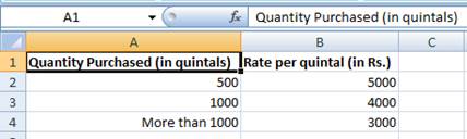
Coffee beans can be purchased according to this price schedule:

For the first 500 Quintal, Rs.5000 per quintal

For the next 1000 quintal, Rs 4000 per quintal

For anything beyond 1000, Rs 3000 per quintal

Create a spreadsheet model that will calculate the total price of buying x quintals of coffee, where x is a number to be entered into a cell on the spreadsheet. (x = 800, x= 1200, x = 300).

STEP 1

Create a table array indicating the rates of coffee beans at different levels of quantity purchased, or simply, the rate list.

STEP 2

Create the output table, where quantity purchased is a variable input and the output is the total cost of the purchase, subject to the rate list created above.

STEP 3

Use ‘IF’ function, as shown below, to model the total cost of coffee.

Case 1 - What-If-Analysis

WHAT-IF Scenarios - Create Different Scenarios

BOOK STORE                                 

"Assume you own a book store and have 1000 books in storage. You sell a certain % for the highest price of 2500 and a certain % for the lower price of 100."                                            

1.    If you sell 60% for the highest price, revenue will be:-------------                                    

2.    WHAT-IF you sell 70% of highest priced book?                   

3.    WHAT-IF you sell 80% of the highest priced book?             

You can simply type in a different percentage (books sold) into cell XX (E9) to see the corresponding result of a scenario (revenues) in cell YY(D14). OR, use what-if analysis to easily compare the results of different scenarios.

WHAT-IF Analysis

1. On the Data tab, click What-If Analysis and select Scenario Manager from the list.

2. Add a scenario by clicking on Add

3. Type a name (Highest price 60%), select the corresponding cell XX (E9 % sold for the highest price) for the Changing cells and click on OK.

4. Enter the corresponding value 0.6 and click on OK again.

5. ADD other scenarios – 70%, 80%, 90% by repeating steps 3 to 5

Note: to see the result of a scenario, select the scenario and click on the Show button. Excel will change the value of cell C4 accordingly for you to see the corresponding result on the sheet.

SUMMARY

Step 6:  Click the Summary button in the Scenario Manager.

Step 7: Select cell YY (D14:  total revenues) for the result cell and click on OK.

Step 8: RESULTS

Conclusion: if you sell 70% for the highest price, you obtain total revenue of: 1780000.

If you sell 80% for the highest price, you obtain total revenue of: 2020000

Excel's Goal Seek

What if you want to know how many books you need to sell for the highest price, to obtain a total profit of exactly 1060000?

1.    On the Data tab, click What-If Analysis, Goal Seek.

The Goal Seek dialog box appears.

2.    Select cell E9 (YY)

3.    Click in the 'To value' box and type 1060000

4.    Click in the 'By changing cell' box and select cell D14 (XX).

5.    Click OK.

RESULT:  You need to sell 40% of the books for the highest price to obtain a total profit of exactly 1060000.

WHAT-IF using Data Tables

Data Tables in Excel

A Data Table is very useful when we have to see the results by altering input variables. Following example illustrates an example of using data table to find out the profit by varying selling price of a product.

Suppose you are a manager in a manufacturing company which produces product P. The demands for Product P are 120 units per week at $85 per unit. The overhead (fixed) cost is around $3500. P requires two raw materials: Steel Widget and Rubber Gasket. Steel Widget costs $20.00 and Rubber gasket is $12.00. You are going to decide how many Ps to make given:

a. To break-even (the net profit is zero)                                                                                             

b. In order to make a profit of $20000                                                                                              

c. If you have a limitation of manufacturing 200 products only and want a minimum profit of 12000, what would be your selling price?

Answer:

A and B can be solved using “Scenario manager” and “Goal Seek” methods of WHAT-IF analysis that was discussed in my earlier posts.

To solve C. We can use DATA TABLE.

Step 1: Enter Number of Products in Cell F14, Selling Price in J14. Calculate Total cost, Total Revenue and Net Profit using appropriate formulas.

Step 2: Prepare a Table first by entering Selling price on each columns (O24 to S24) and product on the rows (M24:M32) as shown below:

Step 3: In Cell D18 enter, reference to the Net Profit cell (N18) as shown below. Cell N24 should have 2860 value (Net profit).

Step 4: Select the Table N23:S30 as shown.

Step 5: From the Excel menu bar, click on Data
Step 6: Locate the Data Tools panel
Step 7: Click on the "What if Analysis" item
Step 8: Click on “Data Table”

Step 9: You will get this window

Step 10: Enter the row and column values. In Column input cell, enter NetProfit cell reference = N18.

Step 11: In Row Input cell, enter selling price cell reference:
Step 12: In Column Input Cell, enter product manufactured cell reference:

Step 13: Enter OK to get the complete Table with Netprofit Values filled.

Step 14: In the table go horizontal on Product 200 row (N30) to get the Net Profit you are looking for (12000). You will find this value under “selling price” of 110.

Conclusion: With a limitation of manufacturing capacity of 200, expecting a Net profit of around 12000, selling value of the product will be 110.